ABOUT SSM
This page explains the state space model and how to estimate its parameters from observed time series data. See our publication [1] and Hirose et al. (2008) [2] in REFERENCE for more details about the model and its estimation.
Links inside this page:
Model
Estimation
Suppressing Oscillating Prediction of Short Time Point Data
Selecting Model and Size of Dimensions
Gene Network Structure
Gene Expression Clustering with Modules
Extracting Differentially Regulated Genes with P Value Calculation
Model
The state space model (SSM) is defined as follows:
x n = F x n − 1 + v n , v n ~ N (0, Q ) [System model]
y n = H x n + w n , w n ~ N (0, R ) [Observation model]
where
p : number of genes (observation variables).
k : size of system dimensions (number of modules). Generally, k < < p is assumed.
x n : ( k )-state vector (variables) at time n .
F : ( k , k )-system transition (coefficient) matrix.
v n : system noise that follows the normal distribution N (0, Q ) .
y n : ( p )-observation vector (variables) at time n .
H : ( p , k )-system-to-observation coefficient matrix.
w n : observation noise that follows the normal distribution N (0, R ) .
We employ the following constraints for the model identifiability.
1. L = H ' R−1 H is diagonal.
2. Q = I .
Fig. 1 shows a graphical image of the state space model.
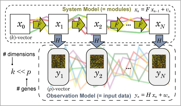
Fig. 1: Graphical image of the state space model.
Estimation
SiGN-SSM estimates parameters ( H, F, R, x0 ) described above from the observed time series gene expression profiles by the EM algorithm where x0 represents the estimated initial state vector (variables). The EM algorithm starts with randomly generated initial values (model parameters), updates the parameters so that the log-likelihood of the model gets increased, and stops when the log-likelihood cannot be improved any more. The EM algorithm can estimate only the local optimal parameters. Therefore, the algorithm needs to perform the estimation many times with the different randomly generated initial values to obtain the better parameters. We recommend to iterate the EM algorithm more than 100 times. SiGN-SSM can perform this in parallel.
As options, the parameter x0 can be fixed to zero (i.e. do not estimate x0 ). The observation noise parameter R can be either R = diag(r 1, ..., r p ) or R = r I .
In addition to the parameters described above, SiGN-SSM produces the following matrices and vectors after the estimation:
D = L −1 H ' R −1/2 : ( k, p )-projection matrix that maps from the observation variables to the system variables.
H E[ x n | y n − 1 ( j ) ] : ( p )-one-step-ahead prediction vector of the observation variables at time n where y n − 1 ( j ) represents the observed data from time 1 to n −1 for the j -th replicate.
H E[ x n | y n ( j ) ] : ( p )-filtering vector of the observation variables at time n where y n ( j ) represents the observed data from time 1 to n for the j -th replicate.
H E[ x n | y N ( j ) ] : ( p )-smoothing vector of the observation variables at time n where y N ( j ) represents the observed data of the entire time point for the j -th replicate.
E[ x n | y n − 1 ( j ) ] : ( k )-one-step-ahead prediction vector of the state variables at time n where y n − 1 ( j ) represents the observed data from time 1 to n −1 for the j -th replicate.
E[ x n | y n ( j ) ] : ( k )-filtering vector of the state variables at time n where y n ( j ) represents the observed data from time 1 to n for the j -th replicate.
E[ x n | y N ( j ) ] : ( k )-smoothing vector of the state variables at time n where y N ( j ) represents the observed data of the entire time point for the j -th replicate.
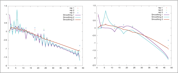
Suppressing Oscillating Prediction of Short Time Point Data
When the algorithm estimates the parameters from short time series
data measured for irregular time intervals,
they are often undesirably highly oscillated (Fig. 2 (left)).
To suppress such spurious patterns, SiGN-SSM implements a novel
constraint on the system transition matrix F along with the
smoothness prior approach.
See our publication [1] and
Wu
Selecting Model and Size of Dimensions
Determining the appropriate size of dimensions (the number of modules) is a difficult task for state space models. After the parameter estimation, the BIC (Bayesian Information Criterion) is calculated with the model parameters, and these BICs are comparable among the estimated models with different sizes of dimensions. Note that the log-likelihood is not comparable among models with different the sizes of dimensions.
Also, the EM algorithm sometimes fails to estimate model parameters. Therefore, it is recommended to estimate model parameters several times (e.g. 100 or more) even for the same size of dimensions and compare them to select the best one by your own. Comparing the prediction plot of the input data is easy way to do this.
Gene Network Structure
After the estimation, ( p, p )-matrix Ψ = D ' L F D represents the coefficients of the estimated gene-to-gene relationships. The ( i, j )-element corresponds to the strength of the estimated relationship from the j-th gene (parent) to the i-th gene (child). The gene network structure can be determined by statistical permutation test that tests the existence of the relationship between every pair of genes using this gene-to-gene coefficient matrix. See Hirose et al. (2008) [2] in REFERENCE for details.
Gene Expression Clustering with Modules
( k, p )-matrix D above represents the mapping from genes to modules. The ( i, j )-element represents the strength of the effectiveness from the j-th gene to the k-th module. Therefore, this matrix can be considered as the clustering of gene expressions based on the estimated state space model.